It is mid July, and you are motor boating through a myriad of islands on the way to your cabin. All is well until the prop hits a rock. You had been through this channel a million times before, and had never hit a rock. What’s Up ?. A few minutes later, as the boat rounds the last island before the cabin, you realise that the trees and shrubs look different. The cleared area in front of the cabin is now covered with shrubs, the shoreline is much farther back than it used to be, and the cabin is starting to sink into the ground !. We all know that water levels change during the year, and that shrubs grow in cleared areas. Some of these changes could be just a natural part of a cycle, but what if they aren’t?.
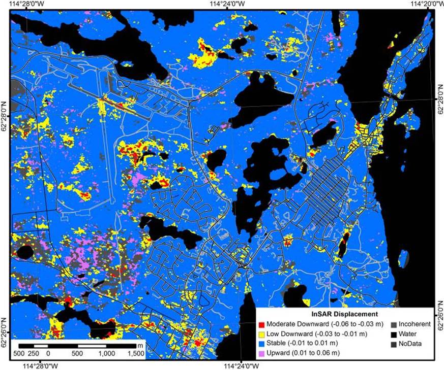
To help understand, the causes and effects of these landscape changes, and if the changes that we are seeing on the landscape are part of a natural cycle or longer-term trend, a team of Federal, Territorial and University scientists are working on a project in the Yellowknife area. Using satellite imagery collected during the past 30 years, and remote sensing techniques we were able to visualize past and on-going changes to the landscape. One of the techniques, called Tasseled Cap Transformation, uses mathematical formulas to calculate values for brightness, greenness and wetness from a satellite image. Brightness represents a measure of reflectance from the surface; features such as bare soil, man-made, and natural features such as concrete, asphalt, gravel, rock outcrops, and other bare areas are considered bright. Greenness is a measure of vegetation; more vegetation is indicated by brighter green areas. Wetness is a measure of surface wetness including soil and plant moisture; wetter areas on the surface indicated by brighter colors on the satellite image. Satellite images spanning the 30 years of available data were analysed for landscape features that represent the Tasseled cap values for Brightness, Greenness, and Wetness. Combining the Tasseled cap values from each separate satellite image, allows the long-term trends in the change of Tasseled cap values for Brightness, Greenness, and Wetness can be observed. In Figure 1, the combined Tasseled cap values for Brightness are represented as shades of red, Greenness in shades of green, and Wetness in shades of blue, with brighter colors representing brighter, greener and wetter areas.

Figure 1
So, what do all the colors mean ?. Using field observations and photos taken from a helicopter, we are able to directly relate the trends (and colors) to observable and recognizable features on the landscape. A photo from the helicopter (Figure 2) over the circled on Figure 1, shows a small inlet with ring of brown vegetation (drying wetlands) and an inner ring of bright green vegetation (new vegetation growth). The combined Tasseled cap colors Brightness, Greenness, and Wetness for this area are yellow and green respectively, suggesting a trend during the past 30 years of yellow areas indicating drying up wetlands, and green areas where there is new vegetation growth. Similarly, areas shown in pink (top left, Figure 1) are presumed to be non-vegetated shallow water areas including dried bogs (Figure 3). A photo of the old and new sections of Highway 3 (Figure 4), shows new vegetation growth on the old section, and paved, wide cleared area with no vegetation, corresponding to light blue and red areas on Figure 1. Areas shown in dark blue, are presumed to be the result of a change to a darker and a wetter forest. The greenish color and banded pattern in the water is a by-product of processing of the imagery and can be ignored.
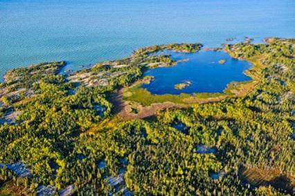
Figure 2
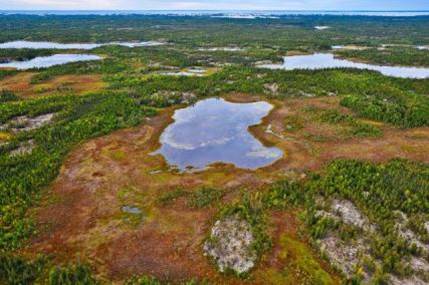
Figure 3
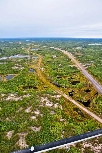
Figure 4
Based on this work, we observed the two major trends shown in the Tasseled Cap Transformation:
1) Apparent lowering of water levels along the shoreline of Great Slave Lake, and in nearby lakes, and shoreline vegetation appears to have expanded in bays. What is not yet fully understood, is the cause of the apparent lowering; it is due to lowering water levels and/or isostatic uplift (land rising after the weight of the glaciers has been removed). Most likely it is a combination of both.
2) Apparent increasing treed vegetation (Dark blue areas on Figure 1). A working hypothesis to explain this trend is that growing conditions have changed such that it is now better for conifer trees such as spruce and jack pine. Additional research work is in progress to understand the increasing treed vegetation.
What do these trends mean in the long-term ?. Are some of these changes just a natural part of a cycle ?. Or – is there any reason to believe that these are the early part of a longer and continuous trend leading to a major climate shift ?.
The data used in this study used satellite imagery that is only available going back 30 years, and does not give any indication of what climatic and landscape changes were occurring in the region 60, 100, 500 or 1000 years ago. Without the long term record, not realistically possible to make long term predictions of the landscape changes into the future. In the short term however, we can predict that water levels will continue to lower and, if growing conditions have recently become better suited to conifer growth, there may be a successional transition from broadleaf forest (beech trees) to conifer trees.
In this project, we have shown landscape change trends in the Yellowknife area. For you, these trends might make it more difficult to navigate to your cabin, and how and where you build your cabin. More importantly, some of the trends in landscape changes observed via the Tasseled Cap Transformation may represent changes which cannot be directly observed. A trend indicating a transition to more-dominate to conifer may also affect the frequency and abundance of forest fires, and may also reflect a change (degradation) in underlying permafrost patterns. The impact of degrading permafrost may have a large impact on a wide range of infrastructure. Anyone who has driven Highway 3 (Yellowknife – Behchoko) will certainly remember a few bumps in the road, the vast majority of which were caused by changes in the permafrost under the highway.
There probably isn’t too much that can be done locally to prevent many of the changes. It is however, important to continue research to understand the underlying causes for the changes. Continued monitoring the changes, will provide useful information to decision makers, for example by showing which areas and terrain features are more sensitive and susceptible to change.
This work is conducted as part of and Natural Resources Canada’s project on Transportation Risk and Climate Sensitivity (TRACS).
Reference: Seventh International Conference and Workshop on the Analysis of Multi-temporal Remote Sensing Images (MultiTemp 2013), Banff, Alberta, Canada, June 25-27, 2013.
Fraser, R.H1, Olthof, I.1, Deschamps, A.1, Pregitzer, M.1, Kokelj, S.2, Lantz, T.3, Wolfe, S.4, Brooker, A.5, Lacelle, D.5, and Schwarz, S.6
(1) Canada Centre for Remote Sensing, Natural Resources Canada, Ottawa, ON
(2) Renewable Resources and Environment, Aboriginal Affairs and Northern Development Canada, Yellowknife, NWT
(3) School of Environmental Studies, University of Victoria, Victoria, BC
(4) Geological Survey of Canada, Natural Resources Canada, Ottawa, ON
(5) Department of Geography, University of Ottawa, Ottawa, ON
(6) NWT Centre for Geomatics, Govt of the Northwest Territories, Yellowknife, NWT